Getting started
getting-started.RmdInstall package
# install devtools packages
if (!require(devtools)) install.packages("devtools")

# load devtools package
library(devtools)

# install mapac package from gitlab
install_git("https://scm.cms.hu-berlin.de/pflugmad/mapac.git",
            quiet = FALSE, force = TRUE)

# Additional packages
install.packages(c("ggplot2", "tidyr", "gt", "flextable", "officer"))Stratified estimation
The function aa_card() estimates map accuracy and area
with a stratified estimator using the map classes as strata (Card,
1982). In this example, we use a data set from Olofsson et al. (2013), a
paper that also describes the method in more detail. The example data is
a list of the following items:
-
reference: a vector of reference labels -
map: a vector of map labels -
h: stratum names associated withw -
w: stratum weights (area proportions) associated with the stratum labelsh -
N_h: stratum sizes (areas) associated with the stratum labelsh -
m: a confusion matrix with the map classes in the rows and the reference classes in the columns.
ex1 <- aa_examples("olofsson")

# confusion matrix
ex1$m
#>                reference
#> map             deforestation forest nonforest
#>   deforestation            97      0         3
#>   forest                    3    279        18
#>   nonforest                 2      1        97

# stratum weights (area proportions)
ex1$w
#> deforestation        forest     nonforest
#>    0.01273585    0.63958045    0.34768370

# stratum names associated with w
ex1$h
#> [1] "deforestation" "forest"        "nonforest"
The aa_card() function takes vectors of reference labels
and map labels as input. If sampling across strata was disproportionate,
you must also provide the stratum weights w (area
proportions) along with the corresponding stratum names h.
These weights are used to adjust the confusion matrix to account for
unequal sampling probabilities. If w and h are
not provided, the function assumes proportional sample allocation across
strata (i.e., equal selection probabilities). This applies to cases such
as simple random sampling or stratified sampling where the sample sizes
within strata are proportional to the stratum sizes.
ex1result <- aa_card(ex1$reference, m = ex1$map, w = ex1$w, h = ex1$h)Instead of providing the stratum names in the h
argument, you can also provide the stratum weights as a named vector in
w.
map_area <- c(deforestation = 22353, forest = 1122543, nonforest = 610228)
w <- map_area / sum(map_area)
w
#> deforestation        forest     nonforest
#>    0.01273585    0.63958045    0.34768370
We can also call aa_card() with the confusion matrix and
the stratum weights.
ex1result <- aa_card(ex1$m, w = ex1$w)When the strata are different from the map classes
Stehman (2014) provides an estimator for the case when the sampling strata are different from the map strata. To illustrate this method, we are going to use the data from Stehman (2014). The data set is a list of the following items:
-
reference: a vector of reference labels -
map: a vector of map labels -
stratum: a vector of stratum labels -
h: a vector of stratum labels associated with the stratum sizesN_h -
N_h: stratum sizes (areas) associated with the stratum labelsh
ex2 <- aa_examples("stehman2014")

# Confusion matrix of the reference and map labels
aa_confusion_matrix(ex2$reference, ex2$map)
#>    reference
#> map A B C D
#>   A 6 1 1 0
#>   B 4 9 3 0
#>   C 0 1 3 2
#>   D 0 1 2 7

# Stratum labels
ex2$h
#> [1] "1" "2" "3" "4"

# Stratum sizes
ex2$N_h
#> [1] 40000 30000 20000 10000
The corresponding function in the mapac package is
aa_stratified(). The function accepts three vectors of
labels (stratum, reference, map) and information on the stratum labels
h and sizes N_h (number of pixels, area, or
area proportion). In our example, there are 4 strata where
h = {"1", "2", "3", "4"}. If the same vector is used for
stratum and map, the estimator yields the same results as the stratified
estimator of the aa_card() function.
ex2result <-  aa_stratified(ex2$stratum, ex2$reference, ex2$map,
                            h = ex2$h, N_h = ex2$N_h)
Results
The result of aa_card() and aa_stratified()
is a list with the following content:
$cm: the adjusted confusion matrix in counts$cmp: the adjusted confusion matrix in area proportion (sums to 1).$stats: User’s (ua) and Producer’s (pa) accuracy and the corresponding standard errors (se) for each class.$accuracy: Overall accuracy and its standard error$area: estimated area proportion and standard errors for each class$fpc: finite population correction factor
ex2result
#> $cm
#>     A    B   C   D
#> A 9.2  1.6 1.6 0.0
#> B 4.8 10.8 3.2 0.0
#> C 0.0  0.8 2.4 1.6
#> D 0.0  0.4 0.8 2.8
#>
#> $cmp
#>      A    B    C    D
#> A 0.23 0.04 0.04 0.00
#> B 0.12 0.27 0.08 0.00
#> C 0.00 0.02 0.06 0.04
#> D 0.00 0.01 0.02 0.07
#>
#> $stats
#>   class        ua     ua_se        pa     pa_se        f1      f1_se
#> 1     A 0.7419355 0.1645627 0.6571429 0.1477318 0.6969697 0.11034620
#> 2     B 0.5744681 0.1248023 0.7941176 0.1165671 0.6666667 0.09354009
#> 3     C 0.5000000 0.2151657 0.3000000 0.1504438 0.3750000 0.13219833
#> 4     D 0.7000000 0.1527525 0.6363636 0.1623242 0.6666667 0.11284328
#>
#> $accuracy
#> [1] 0.63000000 0.08465617
#>
#> $fpc
#> [1] 1 1 1 1
#>
#> $area
#>   class proportion proportion_se
#> 1     A       0.35    0.08225975
#> 2     B       0.34    0.07586538
#> 3     C       0.20    0.06429101
#> 4     D       0.11    0.03073181
#>
#> $adjusted
#> [1] TRUE
Export to text
You can easily export the results as tables in text files.
write.csv(ex2result$cmp, "my_confusion_matrix.csv")HTML
There are a few functions to facilitate visualization and reporting.
The aa_gtable() function creates pretty tables based on the
gt package. The function takes the confusion matrix with
conditional formats. You can incorporate the tables in R markdown or
save them in HTML format via the out_file argument.
| Map class |
Reference class (area %)
|
Σ
|
Accuracy
|
||||||
|---|---|---|---|---|---|---|---|---|---|
| A | B | C | D | Map | Ref. | Producer's | User's | F-score | |
| A | 23.00 | 4.00 | 4.00 | - | 31.00 | 35.00 | 65.71 ± 14.77 | 74.19 ± 16.46 | 69.70 ± 11.03 |
| B | 12.00 | 27.00 | 8.00 | - | 47.00 | 34.00 | 79.41 ± 11.66 | 57.45 ± 12.48 | 66.67 ± 9.35 |
| C | - | 2.00 | 6.00 | 4.00 | 12.00 | 20.00 | 30.00 ± 15.04 | 50.00 ± 21.52 | 37.50 ± 13.22 |
| D | - | 1.00 | 2.00 | 7.00 | 10.00 | 11.00 | 63.64 ± 16.23 | 70.00 ± 15.28 | 66.67 ± 11.28 |
Overall accuracy = 63 ± 8.47 |
|||||||||
You can choose between three different types of confusion matrices: count, proportion, and percent.
cm <- aa_gtable(ex2result, type = "proportion",
                caption = "Confusion matrix (area proportion)")
cm| Confusion matrix (area proportion) | |||||||||
| Map class |
Reference class (area proportion)
|
Σ
|
Accuracy
|
||||||
|---|---|---|---|---|---|---|---|---|---|
| A | B | C | D | Map | Ref. | Producer's | User's | F-score | |
| A | 0.23 | 0.04 | 0.04 | - | 0.31 | 0.35 | 65.71 ± 14.77 | 74.19 ± 16.46 | 69.70 ± 11.03 |
| B | 0.12 | 0.27 | 0.08 | - | 0.47 | 0.34 | 79.41 ± 11.66 | 57.45 ± 12.48 | 66.67 ± 9.35 |
| C | - | 0.02 | 0.06 | 0.04 | 0.12 | 0.20 | 30.00 ± 15.04 | 50.00 ± 21.52 | 37.50 ± 13.22 |
| D | - | 0.01 | 0.02 | 0.07 | 0.10 | 0.11 | 63.64 ± 16.23 | 70.00 ± 15.28 | 66.67 ± 11.28 |
Overall accuracy = 63 ± 8.47 |
|||||||||
If you have long class names, it may be useful to use numbers in the column header.
cm <- aa_gtable(ex2result, col_numbers = TRUE, rm_zero = TRUE)
cm| Map class |
Reference class (area %)
|
Σ
|
Accuracy
|
||||||
|---|---|---|---|---|---|---|---|---|---|
| 1 | 2 | 3 | 4 | Map | Ref. | Producer's | User's | F-score | |
| A | 1 | 23.00 | 4.00 | 4.00 | - | 31.00 | 35.00 | 65.71 ± 14.77 | 74.19 ± 16.46 | 69.70 ± 11.03 |
| B | 2 | 12.00 | 27.00 | 8.00 | - | 47.00 | 34.00 | 79.41 ± 11.66 | 57.45 ± 12.48 | 66.67 ± 9.35 |
| C | 3 | - | 2.00 | 6.00 | 4.00 | 12.00 | 20.00 | 30.00 ± 15.04 | 50.00 ± 21.52 | 37.50 ± 13.22 |
| D | 4 | - | 1.00 | 2.00 | 7.00 | 10.00 | 11.00 | 63.64 ± 16.23 | 70.00 ± 15.28 | 66.67 ± 11.28 |
Overall accuracy = 63 ± 8.47 |
|||||||||
Alternatively, you can provide a different set of class names. You can also turn of cell colors.
cm <- aa_gtable(ex2result, col_numbers = TRUE, cell_colors = FALSE,
                class_labels = c("u", "v", "x", "y"))
cm| Map class |
Reference class (area %)
|
Σ
|
Accuracy
|
||||||
|---|---|---|---|---|---|---|---|---|---|
| 1 | 2 | 3 | 4 | Map | Ref. | Producer's | User's | F-score | |
| U | 1 | 23.00 | 4.00 | 4.00 | - | 31.00 | 35.00 | 65.71 ± 14.77 | 74.19 ± 16.46 | 69.70 ± 11.03 |
| V | 2 | 12.00 | 27.00 | 8.00 | - | 47.00 | 34.00 | 79.41 ± 11.66 | 57.45 ± 12.48 | 66.67 ± 9.35 |
| X | 3 | - | 2.00 | 6.00 | 4.00 | 12.00 | 20.00 | 30.00 ± 15.04 | 50.00 ± 21.52 | 37.50 ± 13.22 |
| Y | 4 | - | 1.00 | 2.00 | 7.00 | 10.00 | 11.00 | 63.64 ± 16.23 | 70.00 ± 15.28 | 66.67 ± 11.28 |
Overall accuracy = 63 ± 8.47 |
|||||||||
Word documents
The aa_flextable() function creates pretty tables based
on the flextable package. You can incorporate the tables in
R markdown or save them in Word (docx) and HTML format via the
out_file argument.
require(flextable)
require(officer)

cm <- aa_flextable(ex2result, type = "proportion",
                   caption = "Confusion matrix (area proportion)")
cmReference class (area proportion) |
Total |
Accuracy |
|||||||
|---|---|---|---|---|---|---|---|---|---|
Map class |
A |
B |
C |
D |
Map |
Ref |
User's |
Producer's |
F1 |
A |
0.23 |
0.04 |
0.04 |
0.00 |
0.31 |
0.35 |
0.742 ± 0.165 |
0.657 ± 0.148 |
0.697 ± 0.110 |
B |
0.12 |
0.27 |
0.08 |
0.00 |
0.47 |
0.34 |
0.574 ± 0.125 |
0.794 ± 0.117 |
0.667 ± 0.094 |
C |
0.00 |
0.02 |
0.06 |
0.04 |
0.12 |
0.20 |
0.500 ± 0.215 |
0.300 ± 0.150 |
0.375 ± 0.132 |
D |
0.00 |
0.01 |
0.02 |
0.07 |
0.10 |
0.11 |
0.700 ± 0.153 |
0.636 ± 0.162 |
0.667 ± 0.113 |
Overall accuracy = 0.630 ± 0.085 |
|||||||||
To display accuracy in percent, use the scale_accuracy
argument.
cm <- aa_flextable(ex2result, type = "percent", col_numbers = TRUE,
                   scale_accuracy = 100,
                   class_labels = c("u", "v", "x", "y"))
cm
Reference class (area %) |
Total |
Accuracy |
|||||||
|---|---|---|---|---|---|---|---|---|---|
Map class |
1 |
2 |
3 |
4 |
Map |
Ref |
User's |
Producer's |
F1 |
U | 1 |
23.0 |
4.0 |
4.0 |
0.0 |
31.0 |
35.0 |
74.2 ± 16.5 |
65.7 ± 14.8 |
69.7 ± 11.0 |
V | 2 |
12.0 |
27.0 |
8.0 |
0.0 |
47.0 |
34.0 |
57.4 ± 12.5 |
79.4 ± 11.7 |
66.7 ± 9.4 |
X | 3 |
0.0 |
2.0 |
6.0 |
4.0 |
12.0 |
20.0 |
50.0 ± 21.5 |
30.0 ± 15.0 |
37.5 ± 13.2 |
Y | 4 |
0.0 |
1.0 |
2.0 |
7.0 |
10.0 |
11.0 |
70.0 ± 15.3 |
63.6 ± 16.2 |
66.7 ± 11.3 |
Overall accuracy = 63.0 ± 8.5 |
|||||||||
Figures
aa_plot_classes(ex2result)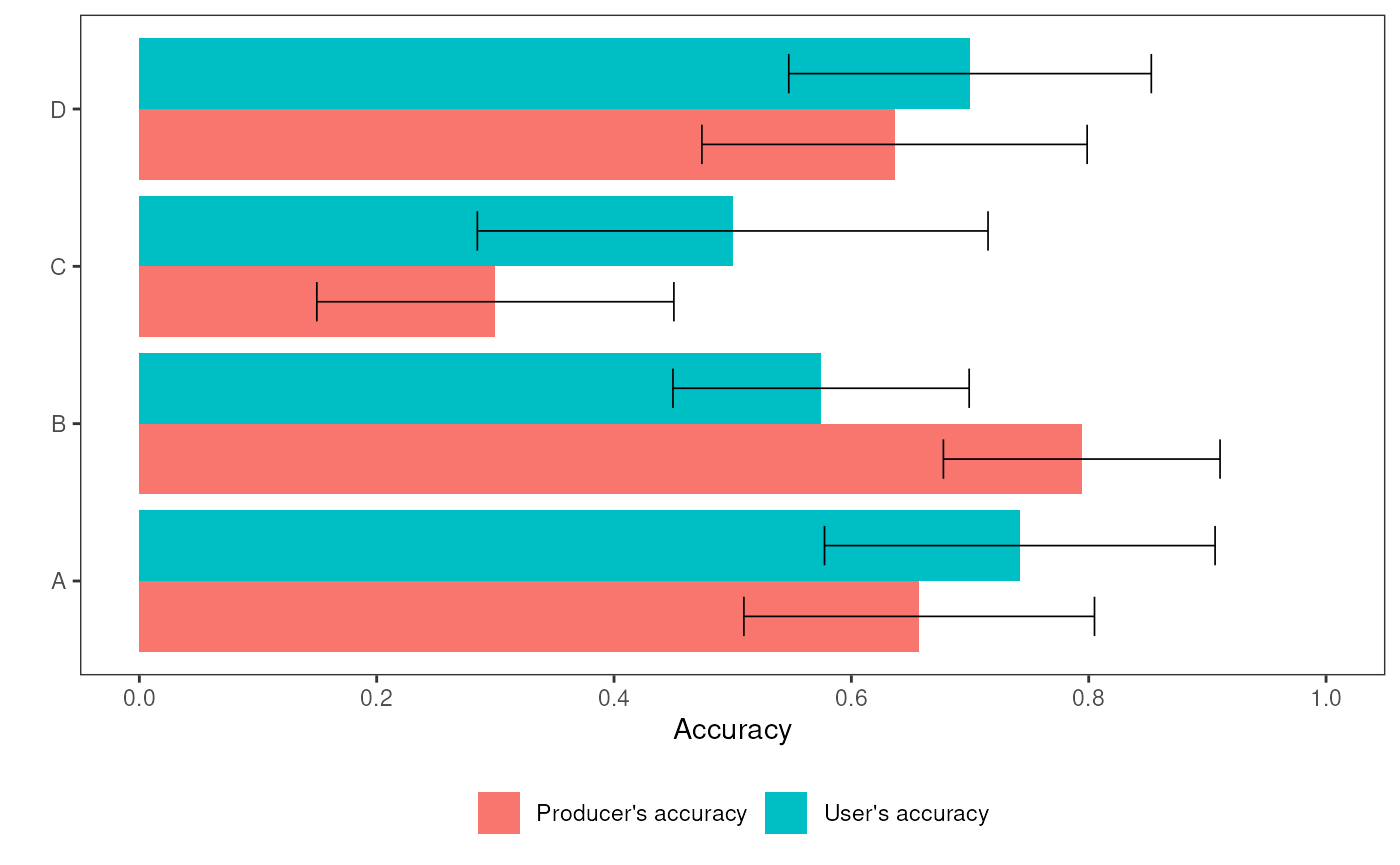
You can save the ggplot as follows:
ggsave("class_accuracy_.png", p, width = 9, height = 6,
       units = "cm", dpi = 300, scale = 2)
References
Card, D.H. (1982). Using known map category marginal frequencies to improve estimates of thematic map accuracy. Photogrammetric Engineering and Remote Sensing, 48, 431-439
Olofsson, P., Foody, G.M., Stehman, S.V., & Woodcock, C.E. (2013). Making better use of accuracy data in land change studies: Estimating accuracy and area and quantifying uncertainty using stratified estimation. Remote Sensing of Environment, 129, 122-131
Stehman, S.V. (2014). Estimating area and map accuracy for stratified random sampling when the strata are different from the map classes. International Journal of Remote Sensing, 35, 4923-4939